|
Kiso Schmidt Plate Digitized Data (KSP) Astrometric Calibration
(Dec.2019)
Notes
(1) SMOKA astrometric calibration is done for a whole area on the plate,
then accurate calibration is found to be difficult.
If you want more accuracy, we recommend the partial area calibration by yourself.
(2) There are several difficulties in the determination of the centers of stars;
the centers of line-shaped stars in "comet" plates are not well-defined,
the centers of stars in Objective Prism plates cannot be well-defined, and
multi-exposure plates (MUL2,MUL3) and sub-beam-prism plates (SB) lead mis-matching of Std.Stars.
2019-11-28
Results of the astrometric calibration are released for 5542 plates.
(1) Astrometric Calibrated Data:
The astrometric calibrated files are updated their FITS header WCS keywords
(CRVAL1, CRVAL2, CRPIX1, CRPIX2, CD1_1, CD1_2, CD2_1, and CD2_2)
and RA2000 and DEC2000,
and keywords about fitting results ( WCSNSTAR, WCSRESID, and WCSFLAGS ) are added;
WCSNSTAR : Number of adopted Std.Stars.
WCSRESID : Mean fitting residuals (arcsec).
WCSFLAGS : Distribution of adopted Std.Stars (6characters).
           1st.char. : W,V  min.value of X-coordinate >= 2/4,1/4 of X-size
           2nd.char. : W,V  max.value of X-coordinate <= 2/4,3/4 of X-size
           3rd.char. : W,V  min.value of Y-coordinate >= 2/4,1/4 of Y-size
           4th.char. : W,V  max.value of Y-coordinate <= 2/4,3/4 of Y-size
           5th.char. : M,N  center of gravity of X-coordinate <= 2/8,3/8 of X-size
                     : P,Q  center of gravity of X-coordinate >= 6/8,5/8 of X-size
           6th.char. : M,N  center of gravity of Y-coordinate <= 2/8,3/8 of Y-size
                     : P,Q  center of gravity of Y-coordinate >= 6/8,5/8 of Y-size
(2) Calibration Methods:
Star extraction program : SExtractor2.19.5
Standard stars catalog : UCAC4 with proper motions
1st.STEP Matching/Fitting program : imwcs in wcstools3.9.5
2nd. and 3rd. STEP Fitting program : minpack.lm on R-3.5.2
Step.A : extract stars with SExtractor.
Step.B : Match/Fit Std.Stars with wcstools.
Step.C : Fit Std.Stars using the Step.B match list with "nls.lm" in "minpack.lm" package of R. (#)
Fit is done two times through 5 arcsec rejection.
Step.D : Match using the Step.C fitting parameters with threshold 10arcsec, then
Fit Std.Stars with "nls.lm" in "minpack.lm" package of R. (#)
Fit is done two times through 3 or 5 arcsec (*) rejection.
(#) Fitting in Step.C and D (so-called "ARC") is applied to minimize the sum of the value V
         V = sqrt( ( DX - ( cd11*(x-xc) + cd12*(y-yc) ) ) **2 +
                   ( DY - ( cd22*(y-yc) + cd21*(x-xc) ) ) **2    ) )

         where
         TH = asin( sin(dc) * sin(dc0) + cos(dc) * cos(dc0) * cos(ra-ra0) )
         TZ = 90.0 * 3600.0 - TH * dr
         DX = TZ * ( cos(dc) * sin(ra-ra0) ) / cos(TH)
         DY = TZ * ( sin(dc) * cos(dc0) - cos(dc) * sin(dc0) * cos(ra-ra0) ) / cos(TH)
         dr = ( 180.0 * 3600.0 ) / pi
         and
         (ra,dc) is the coordinates of each standard star,
         (x,y)   is the coordinates of each detected star on the plate.

           Fitting parameters are 6 :(ra0,dc0) is a projection center
                                     and (cd11,cd12,cd21,cd22) are CD-matrix elements.
           Shift parameters (xc,yc) are fixed to the image center.
(*) displayed in the residual map for each plate as "2nd. step thres.".
Finally, we only use the information on astrometric calibration of the plates
with adopted Std.Stars >= 300 ( in the case of plates with objective prism >= 100 ).
(3) Characteristics of Calibration:
Fitting Residuals:
Upper and lower horizontal lines correspond to "2nd.step thres." 5 and 3 arcsec, respectively.
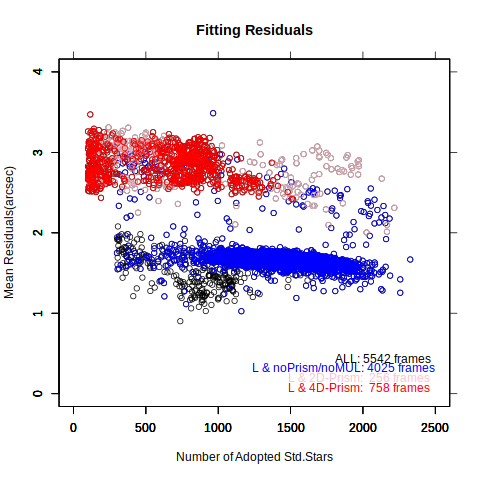 Fig.3-1a
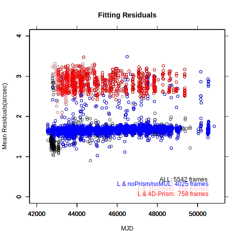 Fig.3-1b
Plate Scales:
X- and Y- axes are those on the files in SMOKA. The scans are done through Y-axis from big to small sides.
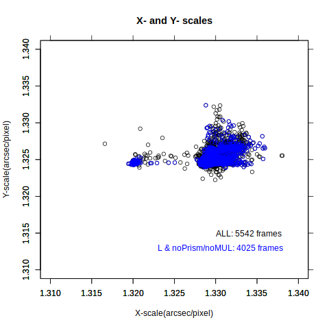 Fig.3-2a
"Variation" may be caused by the telescope or the scanner.
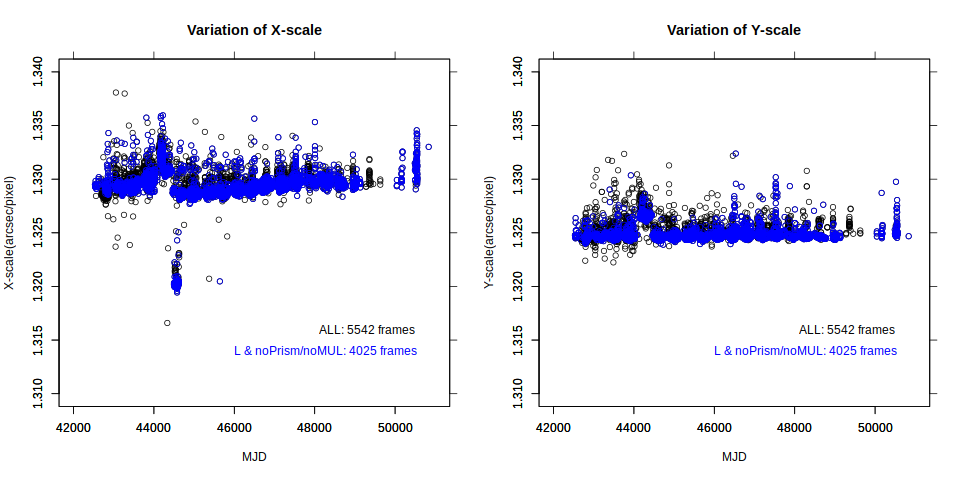 Fig.3-2b
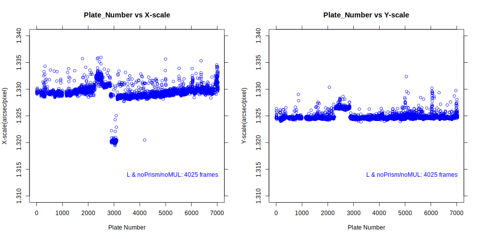 Fig.3-2c
Scan Reproducibility:
The experimental scans are done for (5).
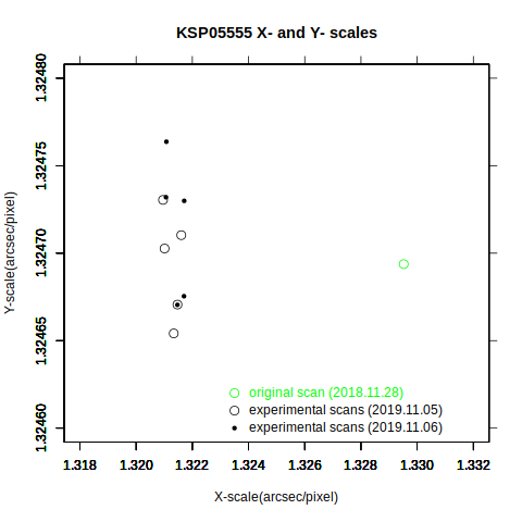 Fig.3-3
(4) Residual Map for each plate:
The map can be seen by clicking the NUMBER in the search results or each THUMBNAIL figure.
The map shows;
matched stars and adopted stars (red) on the image coordinates (upper left)
distribution of residuals (RED|3"|ORN|5"|BLK|8"|BLU) on the image coordinates (upper right)
distribution of residuals (RED|3"|ORN|5"|BLK|8"|BLU) on the celestial sphere projection plane (lower left)
residual vectors (length 100X) on the celestial sphere projection plane (lower right)
with several parameters at the bottom area.
The example figure (KSP05555) :
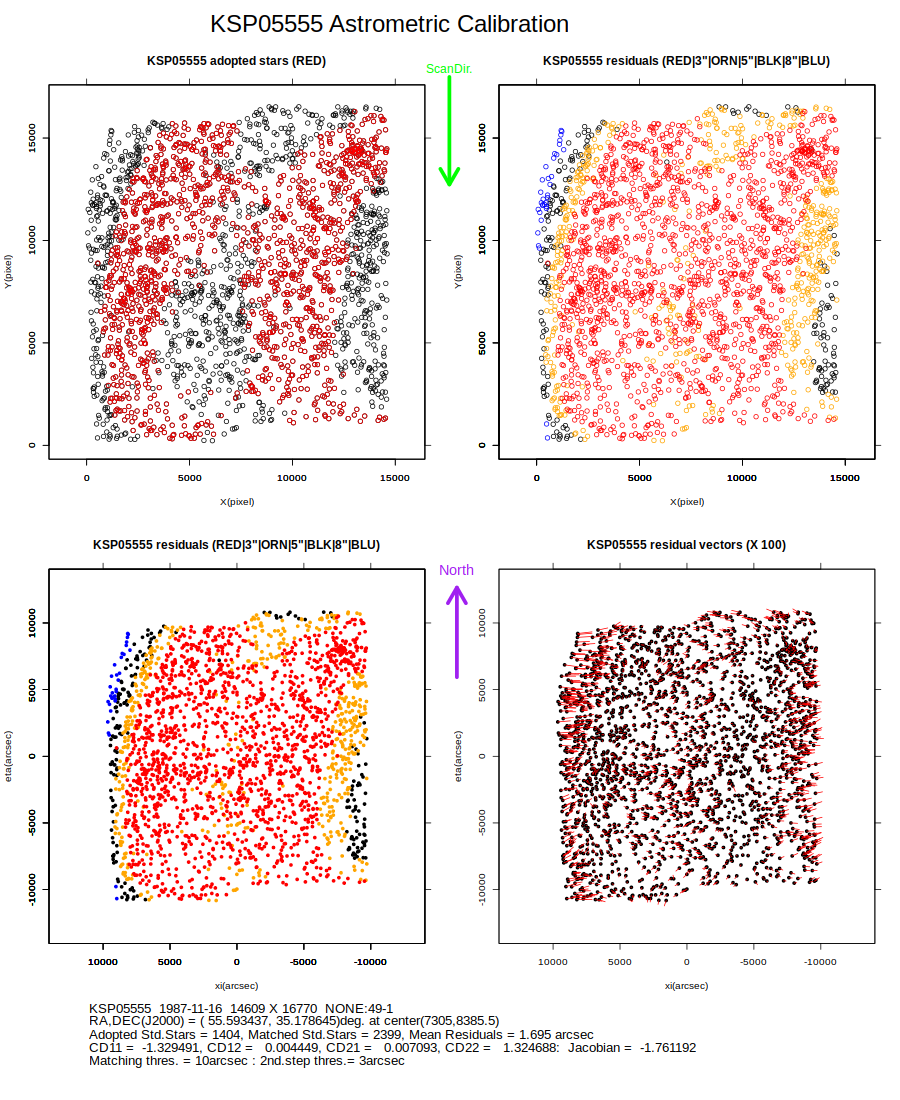 Fig4
Fig4
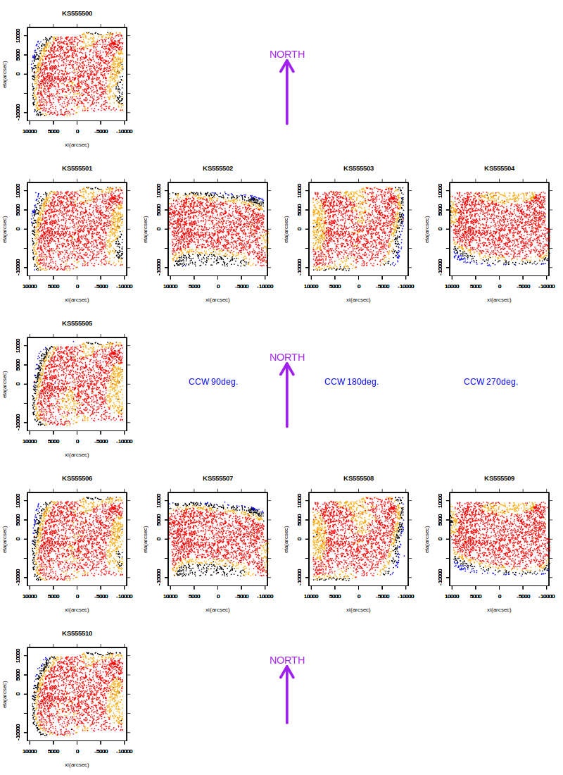
(5) The strange pattern of the Residual Map (see above map):
The residual map for each plate shows the pattern like vertical stripes
(objective prism plates show another pattern).
To examine the source of the pattern, the plate L05555 is scanned with other directions
than the standard direction(0) on the scanner.
  ID       dir. on the scanner     scan date
KS555500     0                    (2018.11.28)  <-- opened by SMOKA
KS555501     0                    (2019.11.05)
KS555502     rotated CCW  90deg.  (2019.11.05)
KS555503     rotated CCW 180deg.  (2019.11.05)
KS555504     rotates CCW 270deg.  (2019.11.05)
KS555505     0                    (2019.11.05)
KS555506     0                    (2019.11.06)
KS555507     rotated CCW  90deg.  (2019.11.06)
KS555508     rotated CCW 180deg.  (2019.11.06)
KS555509     rotates CCW 270deg.  (2019.11.06)
KS555510     0                    (2019.11.06)
The resultant residual maps on the image coordinates are shown in Fig5a.
The residual maps on the celestial sphere projection plane is also shown in Fig5b.
These maps show the patterns are associated with the image coordinates, not with the celestial sphere.
The source of the patterns may be the scanner nonuniformity or fitting programs.
X-direction higher order terms in the fitting formulae may clear the pattern.
These figures are drawn using R.
|